1. Open the file
Click Choose LAS file and select a well-log LAS 1.2 or 2.0 file. Check the displayed well name, sample count, depth range and units. If you are exploring the tool, use the synthetic example above; no real well data is needed.
2. Build four tracks
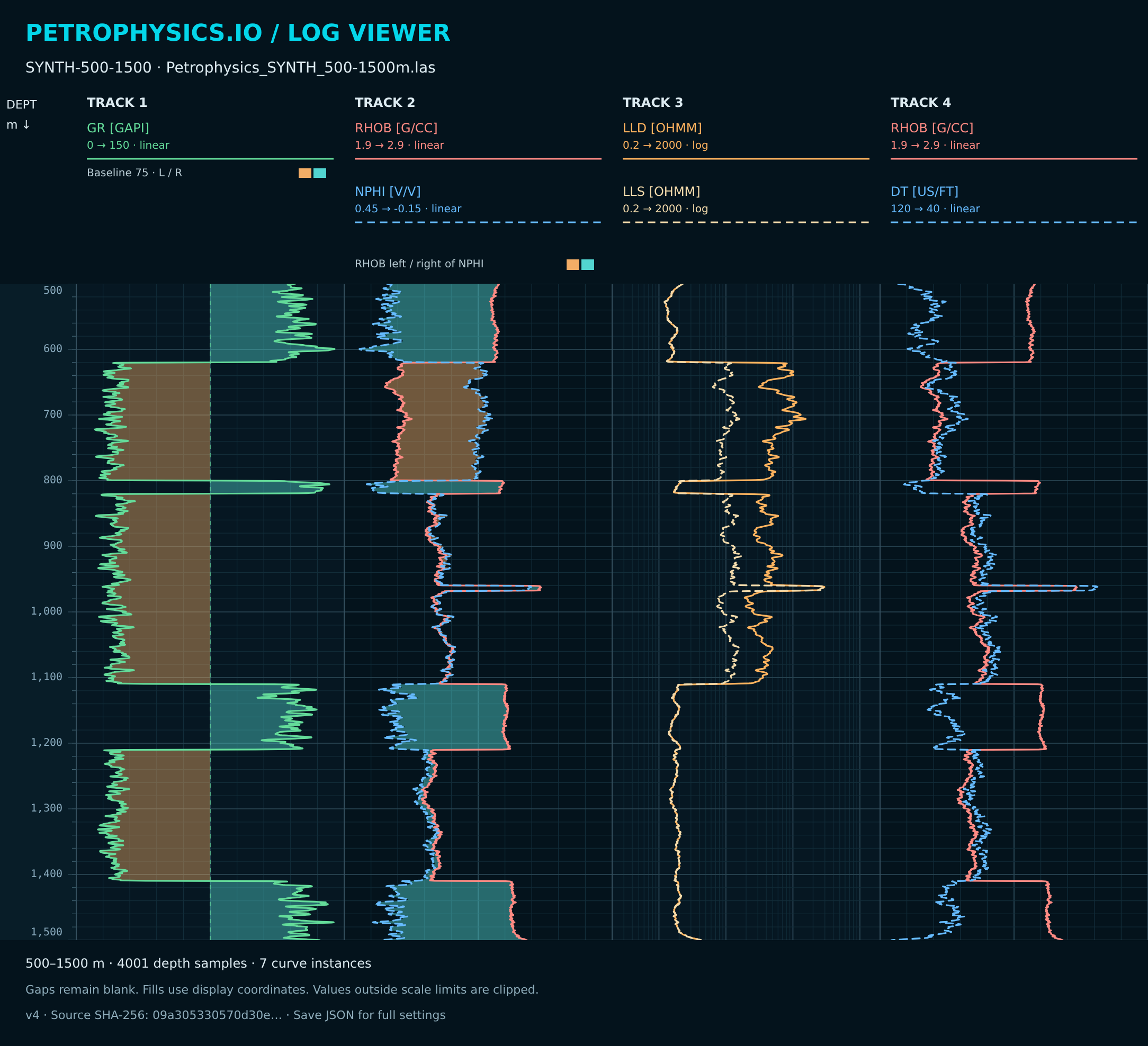
| Track | Curves | Suggested display for this example |
|---|---|---|
| 1 | GR | 0→150 gAPI; baseline 75 |
| 2 | RHOB and NPHI | 1.9→2.9 g/cm³; 0.45→−0.15 v/v |
| 3 | LLD and LLS | 0.2→2,000 Ω·m; logarithmic |
| 4 | RHOB and DT | 1.9→2.9 g/cm³; 120→40 µs/ft |
Drag each curve onto its track. Alternatively, click the curve in the list and then click + on the destination track. Open Track setup to enter the limits. These numbers are for the supplied model: use your file’s units and calibration for other wells.
3. Add fills and choose the interval
For GR, enable the baseline fill, set 75 and choose separate colours for each side. For Track 2, enable a pair fill with RHOB as A and NPHI as B. Set Top 500 and Bottom 1500, then Apply. To inspect the thin cemented interval, use 920–1005 m.
4. Check and export
Click Verify plot and confirm four tracks, seven curve instances and 4,001 depth samples in the full example. Export PNG saves the visible display with scales and legends. Save settings creates its JSON configuration; keep this with the original LAS.
Read the complete Log Viewer reference · Troubleshoot file or settings errors