Download and reproduce
Download the LAS file · Model generator (Python; NumPy + SciPy) · Model QC summary
Settings: four tracks · density–neutron · density–sonic · cement detail. Load the LAS first, then Load settings in the matching tool.
The geological sequence
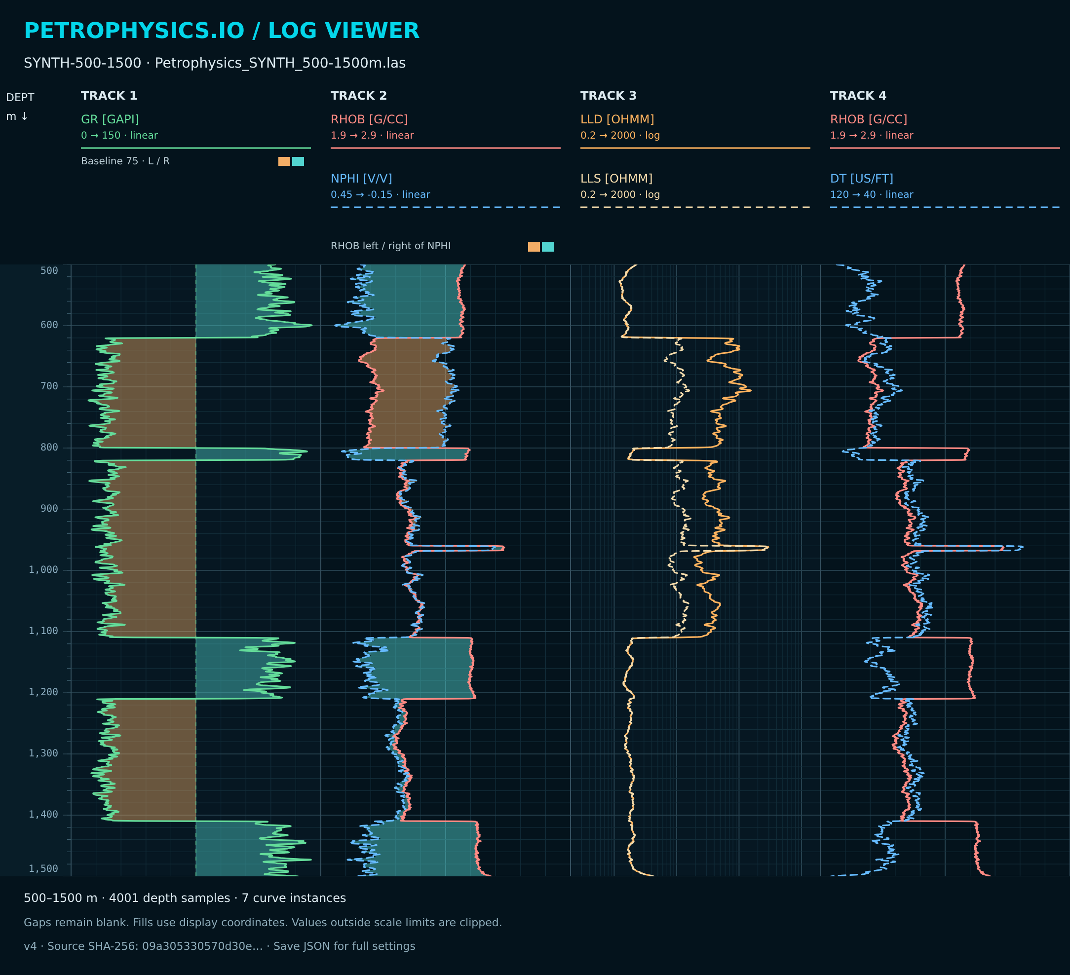
| Depth, m | Assigned layer | FACIES |
|---|---|---|
| 500–620 | Shale | 1 |
| 620–800 | Gas sandstone | 2 |
| 800–820 | Thin shale | 1 |
| 820–960 | Oil sandstone | 3 |
| 960–968 | Tight calcite-cemented sandstone; water-filled | 4 |
| 968–1110 | Oil sandstone | 3 |
| 1110–1210 | Shale | 1 |
| 1210–1410 | Brine sandstone | 5 |
| 1410–1500 | Shale | 1 |
Boundary samples belong to the deeper layer; the final sample at 1,500 m is included. Tool responses are smoothed across boundaries.
Model choices
The generator uses seed 20260929, correlated variations and vertical smoothing. Bulk density mixes quartz/calcite, pore fluid and shale components. Assigned densities are quartz 2.65, calcite 2.71, brine 1.025, oil 0.80 and gas 0.12 g/cm³. These are demonstration inputs, not PVT estimates for the chosen depths.
NPHI uses sandstone units with an illustrative fluid/hydrogen-index response and partial invasion. Resistivity uses assumed Rw=0.12 Ω·m, a=1, n=2, and m=2 for ordinary sands (2.15 for the tight layer), with a small shale-conductivity contribution. Shale resistivity is specified separately. Sonic uses a Wyllie-like fluid baseline and a separate illustrative gas correction; it is not a calibrated acoustic forward model.
The cemented layer has about 2.8% porosity and 45% calcite in its non-shale solid fraction. It is deliberately water-filled: high resistivity is caused by low porosity here. PHIE, SW, VSH, FACIES and ZONE are model truth. They must not be mistaken for properties inferred by the plotting tools.
Expected display checks
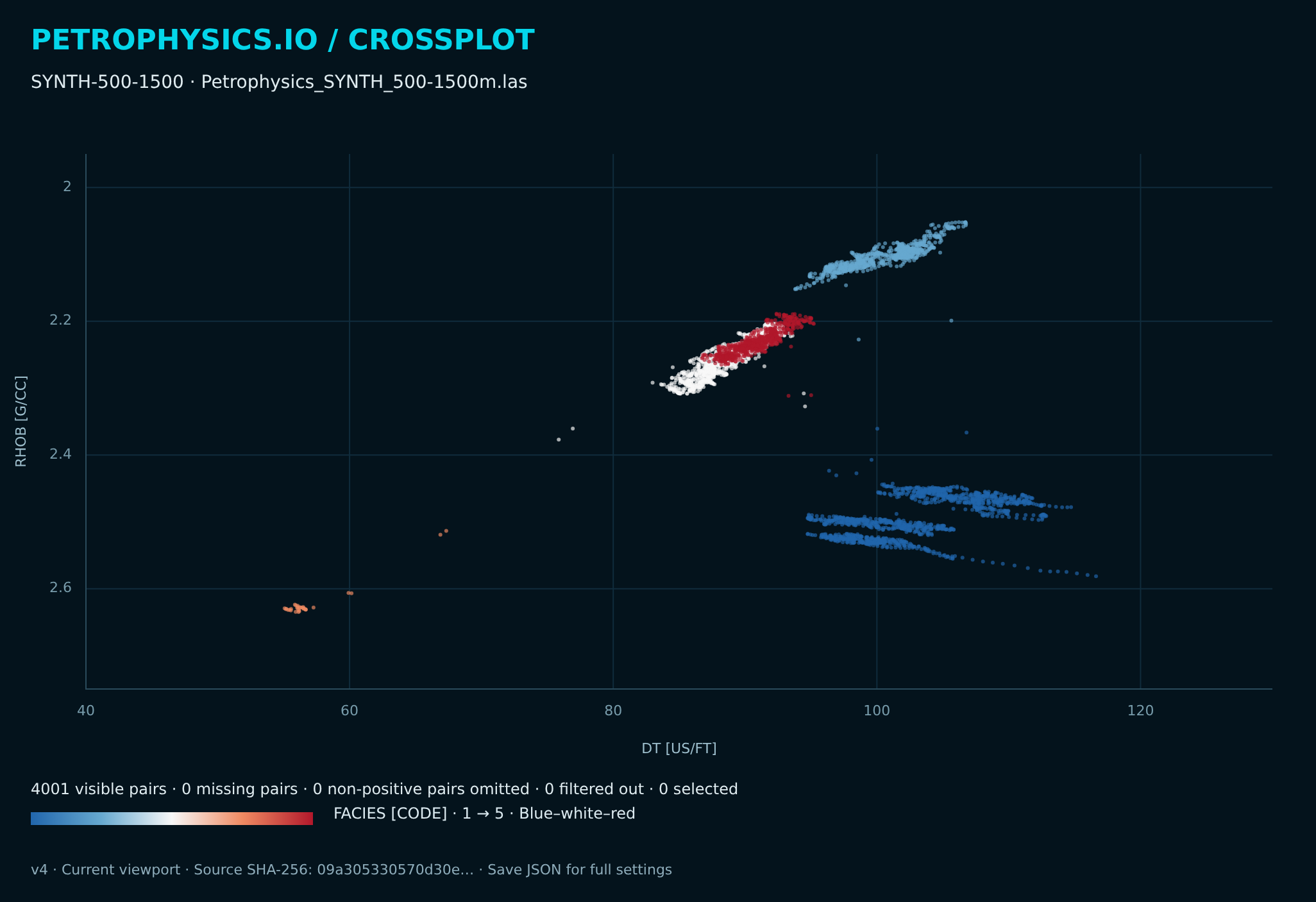
The complete log scene has four tracks and seven curve instances: GR; RHOB/NPHI; LLD/LLS; RHOB/DT. GR uses a baseline of 75 gAPI. Resistivities use log scales from 0.2 to 2,000 Ω·m. Both crossplots have 4,001 numeric pairs; configured limits may clip points, so check visiblePairs separately.
References and limits
SLB: Measuring Porosity Downhole; SLB: sandstone-compatible scale; US EPA: Acoustic Logging. These explain response principles; the generator’s numerical parameters are our illustrative choices.
Use the supplied LAS for exact reproduction. Re-running the generator under different numerical-library versions can change rounding; a different file fingerprint will require newly saved settings.