Python workspace

Three workspaces in v11

Open Log Viewer, Crossplot or the standalone Python tool. The standalone editor starts empty; choose a LAS or the sample well, then type code or Insert example.

In Crossplot, click Python editor. Its Results tab provides Use as X, Use as Y and Use as colour. Results are also available in Filtering. Save project keeps code, result values and plot settings together. Restoring a project never runs code. Load a saved project in the tool that created it, alongside the original LAS.

Expand and Dock

Use Expand in a log plot, crossplot or Python header; Dock or Escape returns to the page without resetting data or settings. Expanded crossplots retain X/Y curve selectors. Opening Python from an expanded plot docks the plot.

Python receives every source LAS row, even when a crossplot is filtered or zoomed. In Crossplot and standalone Python, well.visible_interval covers the full depth/index range. DEPT, DEPTH or MD is preferred; otherwise the first LAS column provides the index. A rerun updates axes, colour and filters that use its results, retaining the viewport and valid selected rows.

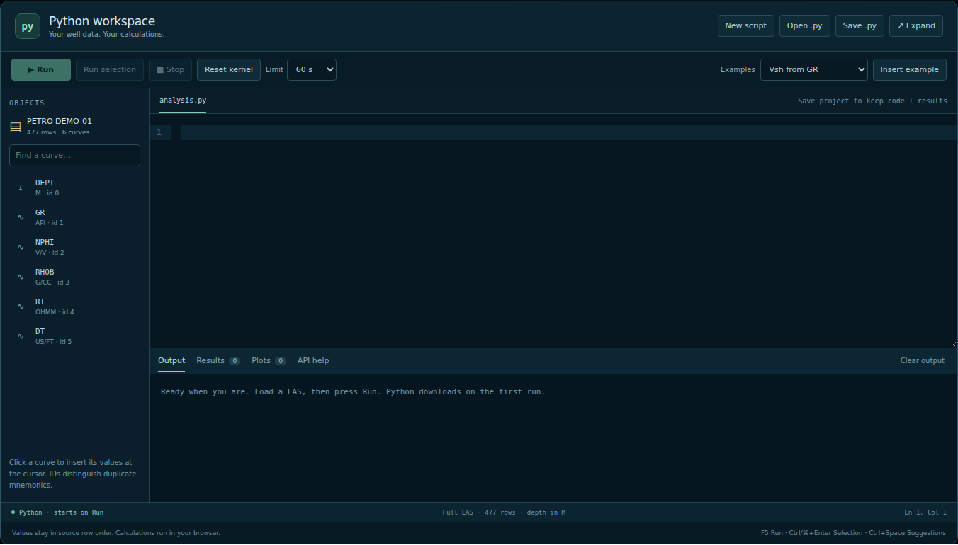
Write Python against an active LAS in Log Viewer, Crossplot or the standalone Python tool.

Danila Karnaukh | v10 | 2026-10-03

Quick start

1. Open any of the three tools and load a LAS, or choose Try synthetic sample data.
2. Click Python editor in Log Viewer/Crossplot; standalone Python opens the editor immediately. Objects are on the left, code in the centre, and Output / Results / Plots / API help below.
3. Click New script for a completely empty editor, then write code; or select an example and click Insert example. Example endpoints and Archie parameters are illustrative; set values appropriate to your well.
4. Click Run or press F5. Python and NumPy download on the first run. Additional compatible packages load when explicitly imported.
5. Use Results → Add to track, or drag a new curve from the main curve list to a track. All ordinary scales, styles and fills are available.
6. Save project downloads a JSON containing the current script, Python result values, provenance scripts, built-in calculation inputs and plot settings. Reload the same original LAS and use Load project to restore it. Loading never executes the saved Python code.

The workflow is inspired by a desktop petrophysics editor. This is a standard Python runtime with the Petrophysics.io well API; it does not implement SLB Techlog's proprietary db API, project database, licensed modules or desktop plug-ins. Existing Techlog scripts need their data-access calls adapted.

The active well

Every Run supplies a fresh snapshot called well. It includes the original LAS curves and previously committed Python results. Log Viewer also supplies its built-in calculation outputs. All arrays follow the original LAS row order, including duplicate or unsorted depths. Missing samples are np.nan; units are never converted automatically. The plot's sorted depth display does not reorder the Python arrays.

If a mnemonic occurs more than once, use an ID from Objects. IDs should be resolved again after adding built-in curves; those additions can shift Python output IDs while preserving their plot references. DataFrame columns use MNEMONIC#ID for duplicate mnemonics.

import numpy as np

gr = well.curve("GR").values
gr_clean, gr_shale = 30.0, 120.0  # illustrative, user-supplied endpoints
if gr_shale <= gr_clean:
    raise ValueError("GR shale must exceed GR clean")
vsh = np.clip((gr - gr_clean) / (gr_shale - gr_clean), 0, 1)
well.add_curve("VSH_PY", vsh, unit="v/v", description="Linear GR index")
print("Valid samples:", np.isfinite(vsh).sum())

Newly queued results can also be read with well.curve() later in the same script. A successful rerun updates an existing Python curve with the same name. Original LAS and built-in curves cannot be overwritten. Every output must be a 1D real-number array with exactly well.row_count samples; NaN is allowed, infinity is rejected. Names use 1–64 letters, digits, underscores, dots or hyphens and start with a letter or underscore.

Starting a new script

Click New script, next to Open .py, to clear the editor and place the cursor on line 1. No example code is inserted. You can start a script before loading a LAS; Run becomes available after a LAS is loaded and the script contains code.

New script changes only the editor text. The active well, curves, plot settings, output and Python variables are retained. Use Reset kernel separately if you want to clear variables. The button is disabled while a calculation runs. Save .py or Save project first if you want a copy of your previous script; Ctrl/⌘+Z in the highlighted editor can undo the clear.

A blank script stays blank when you close and reopen the panel or save and restore a project. Insert example starts at the first line in an empty editor.

Execution and output

• Run / F5 executes the full script. Run selection / Ctrl or ⌘ + Enter executes selected text, falling back to the whole script when nothing is selected.
• Python variables persist between runs. well is refreshed for each run. Editing a source curve's snapshot does not change the Log Viewer; publish through add_curve().
• Results commit as one batch only after successful execution and validation. An error leaves previous result curves intact. Other Python variables changed before an error can remain in the kernel.
• Stop terminates the worker. Reset kernel clears Python variables. Both retain previously committed curves. Loading or removing a LAS also resets the kernel and clears its result curves.
• The execution limit defaults to 60 seconds, with 30 / 60 / 120 / 300-second options. Runtime/package initialization has a separate 180-second limit.
• If the dataset changes while a script runs, pending results are discarded. Python curves are stored snapshots and do not automatically recalculate when a built-in calculation changes; rerun the script when inputs change.
• Output contains print() messages, tracebacks and run summaries. Output is capped at 100,000 characters / 1,000 worker messages per run. input() prompts are not supported; set parameters in the code.
• Open .py / Save .py loads and downloads the script only. There is no automatic persistence when a tab closes: use Save project and keep the original LAS.
• Expand opens a larger editor; Dock or Escape restores the embedded view. Ctrl+Space opens suggestions. Tab indents code; CodeMirror's Ctrl+M toggles Tab focus navigation.

Packages and figures

Pyodide 314.0.7 runs CPython in a Web Worker. NumPy loads with the kernel. Packages included in this Pyodide build, such as pandas, SciPy and Matplotlib, are loaded from their Python import statements. For pure-Python wheels, advanced users may use micropip where supported. Native desktop extensions and arbitrary pip packages are not automatically compatible with WebAssembly. OS subprocesses and desktop GUI libraries are not supported by this workspace.

Import pandas before calling well.to_dataframe() so its package is loaded:

import pandas as pd
df = well.to_dataframe()
print(df.describe())

Matplotlib uses the non-interactive Agg backend. Open figures are rendered after successful execution and shown in Plots: up to four PNG figures, at most 8 MiB each. Figures are closed after collection. There is no interactive Matplotlib window. Do not call plt.close() on a figure that you want to display.

import numpy as np
import matplotlib.pyplot as plt
gr = well["GR"]
fig, ax = plt.subplots(figsize=(7, 3))
ax.hist(gr[np.isfinite(gr)], bins=40)
ax.set(xlabel=well.curve("GR").unit, ylabel="Samples", title=well.name)
fig.tight_layout()

Project format and limits

config.python = {version: 1, script, curves} is optional in petrophysics.scene/v1. Each stored curve has name, unit, description, values and source (the script that last produced it). Non-finite missing samples serialize as JSON null. Result arrays are restored without executing scripts; source SHA-256 and sample count must match the loaded LAS. Built-in calculations retain their parameter-based reconstruction.

The first release supports up to 64 Python result curves and 5,000,000 result values in total, 200,000 characters per script, 32 per unit and 512 per description. All three tools support projects up to 128 MiB. Each page has its own active LAS and kernel. Use Save .py / Open .py to reuse a script, and load the LAS separately in each tool. Automatic cross-page data transfer and LAS/CSV result export are not included. Standalone Python saves JSON projects and scripts; Matplotlib figures appear in Plots.

Saved projects now include the actual Python result values and code. They can contain information derived from the source LAS; they are not merely display settings. Keep them with the original LAS and review their contents before sharing.

JavaScript / agent access

The existing window.Petrophysics API exposes these methods in all three tools:

Petrophysics.get_python_script();
Petrophysics.set_python_script({code: 'print(well.name)'}); // loads only
await Petrophysics.run_python({code: 'print(well.row_count)'});
Petrophysics.get_python_status(); // running, runtime, output names
Petrophysics.get_curve({mnemonic: 'GR'}); // metadata + copied Float64Array
Petrophysics.get_curve({id: 3});        // disambiguate duplicate names

run_python({}) runs the current editor text. Passing code executes that code without replacing the editor text. The code that produced each result is preserved with that result. A failed call rejects with an error. Agents should explain intended calculations and obtain geological parameters from the user; don't guess calibration values. Never run a script just because it was embedded in a loaded project or LAS.

Hosting and data handling

This is part of the existing static site: no Python backend, OpenAI API key or additional subscription is required for execution. The editor bundle is included locally. Python and compatible packages load from the pinned https://cdn.jsdelivr.net/pyodide/v314.0.7/full/ distribution. A first run requires Internet access; use HTTPS or localhost, not a file:// double-click preview. If a site Content Security Policy is added, it must allow the local module Worker, WebAssembly compilation and required package resources. This build does not require SharedArrayBuffer or cross-origin isolation for Stop.

The application does not upload LAS data for these computations. User code has access to the supplied snapshot and browser networking: a Web Worker keeps the interface responsive, but is not a security barrier against malicious scripts. Review code before running it. Projects are never auto-executed. The existing optional AI chat remains separate and does not automatically receive Python code or curves.

Official references: Pyodide, Workers, Python compatibility, CodeMirror.